Auditing Allocative Bias

Kate Kenny

CS 0451

In this blog post, we are going to examine algorithmic bias through an audit. Using data from the American Community Survey’s Public Use Microdata Sample (PUMS). I will perform an audit on racial bias in a machine learning model that predicts whether or not an individual in employed.To do this, I will begin by downloading data and training a model to make such predictions. Then, we will examine some of the different measures of fairness like predictive parity and error rate before discussing how the model could be biased and what implications that could have in deployment and beyond. This audit will only consider data from New York State.

To begin, let’s download the data and get the problem set up.

from folktables import ACSDataSource, ACSEmployment, BasicProblem, adult_filter
import numpy as np
from matplotlib import pyplot as plt


STATE = "NY"

data_source = ACSDataSource(survey_year='2018', 
                            horizon='1-Year', 
                            survey='person')

acs_data = data_source.get_data(states=[STATE], download=True)


possible_features=['AGEP', 'SCHL', 'MAR', 'RELP', 'DIS', 'ESP', 'CIT', 'MIG', 'MIL', 'ANC', 'NATIVITY', 'DEAR', 'DEYE', 'DREM', 'SEX', 'RAC1P', 'ESR']
features_to_use = [f for f in possible_features if f not in ["ESR", "RAC1P"]]

is_white = acs_data["RAC1P"] == 1
is_black = acs_data["RAC1P"] == 2

acs_data = acs_data[is_white | is_black]
acs_date = acs_data.copy()

EmploymentProblem = BasicProblem(
    features=features_to_use,
    target='ESR',
    target_transform=lambda x: x == 1,
    group='RAC1P',
    preprocess=lambda x: x,
    postprocess=lambda x: np.nan_to_num(x, -1),
)

features, label, group = EmploymentProblem.df_to_numpy(acs_data)

for obj in [features, label, group]:
  print(obj.shape)

(162498, 15)
(162498,)
(162498,)
[1 1 1 ... 1 1 1]

Seperate training and testing data

from sklearn.model_selection import train_test_split
X_train, X_test, y_train, y_test, group_train, group_test = train_test_split(
    features, label, group, test_size=0.2, random_state=0)

Basic Descriptives

Let’s first answer some basic questions about the test data that we are working with. For the sake of this blog, we are going to compare directly Black and white individuals and remove individuals with other listed races from the data frame. This is obviously an incomplete picture of New York’s population but allows us to directly compare and analyze specific racial discrepencies between white individuals and Black individuals. Note that in the group column of the data frame, group 1 represents white individuals and group 2 represents Black individuals. Furthermore, employment status is 1 for an individual that is employed and 0 for an unemployed individual.

import pandas as pd
df = pd.DataFrame(X_train, columns = features_to_use)
df["group"] = group_train
df["label"] = y_train

df.shape[0]
y_train.mean()

0.4661840951399252

There are 129,998 individuals in this data set. Of those individuals, the proportion of people with the target label 1 (employed individuals) is .46618.

df.groupby("group")["label"].mean()

group
1    0.474091
2    0.420689
Name: label, dtype: float64

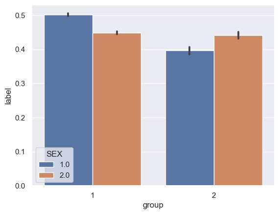
Within each group, there is a difference in the proportion of individuals with the target label 1. Among white individuals (group 1), the proportion is .474091 and among Black individials (group 2) the proportion is .420689. This is a difference that is likely the result of many historical factors and centuries of systemic racism in the United States and certainly deserves much more focus than is covered in the scope of this blog post. It is important to note that as the base rates for white and Black individuals differ, it is impossible for our model to achieve callibration and error rate balance. However, for now let’s continue. The following table is the result of breaking the data down by race and sex. Note that in the SEX category, 1.0 refers to male and 2.0 refers to female.

import seaborn as sns

intersectional = df.groupby(["group", "SEX"])["label"]
sns.set_theme()

sns.barplot(data=df, x="group", y="label", hue="SEX")

#CHANGE LABELS

<AxesSubplot: xlabel='group', ylabel='label'>

In this chart, it is interesting that white women and Black women have very similar rates of employment. However, white men have a higher rate of employment compared to white women and the opposite is true for Black men and women.

Build and train model

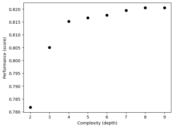
The model we are going to use is the Scitkit-Learn Decision Tree Classifier. Before finalizing our model, we can use cross validation to select the depth for the model in order to balance a high training score and limiting overfitting.

from sklearn.tree import DecisionTreeClassifier, plot_tree
from sklearn.pipeline import make_pipeline
from sklearn.preprocessing import StandardScaler
from sklearn.metrics import confusion_matrix

#cross validation to choose depth
from sklearn.model_selection import cross_val_score
np.random.seed(12345)

fig, ax = plt.subplots(1)

for d in range(2, 10):
    T = DecisionTreeClassifier(max_depth = d)
    m = cross_val_score(T, X_train, y_train, cv = 10).mean()
    ax.scatter(d, m, color = "black")
    # ax.scatter(d, T.score(X_test, y_test), color = "firebrick")

labs = ax.set(xlabel = "Complexity (depth)", ylabel = "Performance (score)")

0.8037772249581154
0.8101165062594978
0.7835820895522388

It seems like a depth of 4 could be ideal as the score improvement slows down significantly when the depth continues to increase beyon 4. So, to prevent against overfitting it seems that 4 is the best choice. Given that, let’s train our model on the available data before moving into testing.

model = make_pipeline(StandardScaler(), DecisionTreeClassifier(max_depth = 4))
model.fit(X_train, y_train)

Pipeline(steps=[('standardscaler', StandardScaler()),
                ('decisiontreeclassifier',
                 DecisionTreeClassifier(max_depth=4))])

In a Jupyter environment, please rerun this cell to show the HTML representation or trust the notebook.
On GitHub, the HTML representation is unable to render, please try loading this page with nbviewer.org.

Testing and Audit

Now that we have trained a model, let’s use it on test data and do an audit surrounding the accuracy, fairness, and allocative bias in the results.

y_hat = model.predict(X_test)

print("Overall accruacy:")
print((y_hat == y_test).mean())

Overall accruacy:
0.8151692307692308
Accuracy for white individuals
0.8174079284348735
Accuracy for Black individuals
0.8021770985974461

Initially, our model has an accuracy of .815 overall. Next, let’s consider the general confusion matrix for this test data.

from sklearn.metrics import confusion_matrix

#calculate false neg, false pos rates
confusion_matrix(y_test, y_hat, normalize = "true")

array([[0.79528736, 0.20471264],
       [0.16192053, 0.83807947]])

The false negative rate of our model is .1619 and the false positive rate of our model is .2047.

Next, let’s consider some of the mathematical measures of fairness that we have been working with in the context of this model. We can measure the calibration, error rate balance, and statistical parity.

#calculate PPV
np.sum(y_test) / np.sum(y_hat)

0.9311216624529814

The overall positive predictive values (PPV) of the model is .9311.

Now that we have some overall measures, let’s dive deeper into the different measures of accuracy by group.

print("Accuracy for white individuals")
print((y_hat == y_test)[group_test == 1].mean())
print("Accuracy for Black individuals")
print((y_hat == y_test)[group_test == 2].mean())

Accuracy for white individuals
0.8174079284348735
Accuracy for Black individuals
0.8021770985974461

When we group by race above, we can see that the accuracy for white individuals (.8174) is slightly higher than the accuracy for Black individuals (.8023). Next let’s consider the positive predictive value for both groups. This is the number of predicted labels of 1 divided by the actual number of target labels 1. In other words, it’s how often a positive prediction from the model is correct.

print("PPV for white individuals")
print(np.sum(y_test[group_test == 1]) / np.sum(y_hat[group_test == 1]))
print("PPV for Black individuals")
print(np.sum(y_test[group_test == 2]) / np.sum(y_hat[group_test == 2]))

df = pd.DataFrame(X_test, columns = features_to_use)

df["pred_label"] = 1* y_hat.tolist()
df["label"] = y_test.tolist()
df["race"] = group_test.tolist()

df.groupby(["race", "pred_label"])["label"].mean().reset_index(name = "mean")

PPV for white individuals
0.9366807535276843
PPV for Black individuals
0.8967198581560284

	race	pred_label	mean
0	1	False	0.151795
1	1	True	0.787050
2	2	False	0.141214
3	2	True	0.738918

The PPV for white individuals if 4 percentage points higher than that for Black individuals. This means that the model is not perfectly calibrated although the disparity is not that extreme.

#Confusion matrix for Black individuals 
confusion_matrix(y_test[group_test == 2], y_hat[group_test == 2], normalize = "true")

array([[0.78612927, 0.21387073],
       [0.17597627, 0.82402373]])

#Confusion matrix for white individuals
confusion_matrix(y_test[group_test == 1], y_hat[group_test == 1], normalize = "true")

array([[0.79700942, 0.20299058],
       [0.15974612, 0.84025388]])

The false negative rate for Black individuals is .1759 and the false positive rate is .2138. The false negative rate for white individuals is .1597 and the false positive rate is .2138. So this is not an extreme difference but the error rates are not completely balanced.

The model would be calibrated if Black and white individuals who were predicted to be unemployed had the same chance of being unemployed. To calculate this, we want to take all the individuals who were predicted to be unemployed and calculate what percentage actually are by group.

Finally, let’s consider statistical parity. Statistical parity is achieved if a protected group is treated equally by the model as the entire population being considered. So in this context, that would mean Black individuals being predicted to be unemployed with the same accuracy as the general predictions. As calculated above, the overall accuracy is .815. The accuracy for Black individuals is .802. So again, this is a slight difference but there is a discrepency.

Overall, our model seems to have slight bias against Black Individuals using all of our measures of fairness but none of these disparities is as extreme as the example we examined in class. However, that does not mean it is insignificant. Discrimination is compounding and all of these differences can lead to a combined effect of Black individuals being discriminated against by our model.

Further Discussion

Now, let’s consider the broader implications of the model we have created, what contexts that it could be used in, and how any unfairness by different standards could impact individuals when our model is being used. An algorithm that predicts unemployment could be useful to a variety of companies or interests. People renting homes, giving loans, or providing other social services could all be interested in predicting employment status. I could also see such a model being used for backround checks of various kinds, espeically when information on individuals could be limited or collecting employment status is not permitted in the circumstance.

Based on my audit, I think that the impact of my model being deployed by a corportation or the government could perpetuate existing economic inequalities for Black individuals. A model that predicts Black unemployment at a higher rate than white individuals could lead to people already facing systemic oppression being denied opportunities or social services. The model constructwed in this post has slight disc rimination according to each measure of fairness we considered. Although these are all relatively small, they all are unfair towards Black individuals implying that implementing the model on a large scale would have a disparate impact on that population. Small, maybe even statistically insignificant, discrimination in many areas or by many standards adds up and does impact the lives of real people.

Beyond the actual fairness of the model, there are some moral considerations that I would have to take into account before allowing this model to be implemented in the real world. Let’s consider the example of government agencies providing certain social services, housing, health insurance, or other benefits based on whether the model expects an individual to be able to pay for them based on employment status. For example, there have been welfare laws that require employment and I could see this being used to implement similar programs across different social sectors. I personally do not believe it is the job of the government to deny individuals social services or aid if they are unemployed. It would obviously be unfortunate if an individual was denied a service because the model predicted they were unemployed and they were not, but I think the real failure in that instance is making help conditional on employment and only valuing those who “contribute” to society based on capitalist values rather than valuing and prioritizing a social safety net for all.